Cluster Analysis Gets Complicated

This article was published in Marketing Research, spring 2003.

Collinearity is a natural problem in clustering. So how can researchers get around it?

Cluster analysis is widely used in segmentation studies for several reasons. First of all, it’s easy to use. In addition, there are many variations of the method, most statistical packages have a clustering option, and for the most part it’s a good analytical technique. Further, the non-hierarchical clustering technique k-means is particularly popular because it’s very fast and can handle large data sets. Cluster analysis is a distance-based method because it uses Euclidean distance (or some variant) in multidimensional space to assign objects to clusters to which they are closest. However, collinearity can become a major problem when such distance based measures are used. It poses a serious problem that, unless addressed, can produce distorted results.

Executive Summary

Segmentation studies using cluster analysis have become commonplace. However, the data may be affected by collinearity, which can have a strong impact and affect the results of the analysis unless addressed. This article investigates what level presents a problem, why it’s a problem, and how to get around it. Simulated data allows a clear demonstration of the issue without clouding it with extraneous factors.
Collinearity can be defined simply as a high level of correlation between two variables. (When more than two variables are involved, this would be called as multicollinearity.) How high does the correlation have to be for the term collinearity to be invoked? While rules of thumb are prevalent, there doesn’t appear to be any strict standard even in the case of regression-based key driver analysis. It’s also not clear if such rules of thumb would be applicable for segmentation analysis.

Collinearity is a problem in key driver analysis because, when two independent variables are highly correlated, it becomes difficult to accurately partial out their individual impact on the dependent variable. This often results in beta coefficients that don’t appear to be reasonable. While this makes it easy to observe the effects of collinearity in the data, developing a solution may not be straightforward. See Terry Grapentine’s article in the Fall 1997 issue of this magazine (“Managing Multicollinearity”) for further discussion.

The problem is different in segmentation using cluster analysis because there’s no dependent variable or beta coefficient. A certain number of observations measured on a specified number of variables are used for creating segments. Each observation belongs to one segment, and each segment can be defined in terms of all the variables used in the analysis. From a marketing research perspective, the objective in each case is to identify groups of observations similar to each other on certain characteristics, or basis variables, with the hope this would translate into opportunities. In a sense, all segmentation methods are trying for internal cohesion and external isolation among the segments.

When variables used in clustering are collinear, some variables get a higher weight than others. If two variables are perfectly correlated, they effectively represent the same concept. But that concept is now represented twice in the data and hence gets twice the weight of all the other variables. The final solution is likely to be skewed in the direction of that concept, which could be a problem if it’s not anticipated. In the case of multiple variables and multicollinearity, the analysis is in effect being conducted on some unknown number of concepts that are a subset of the actual number of variables being used in the analysis.

For example, while the intention may have been to conduct a cluster analysis on 20 variables, it may actually be conducted on seven concepts that may be unequally weighted. In this situation, there could be a large gap between the intention of the analyst (clustering 20 variables) and what happens in reality (segments based on seven concepts). This could cause the segmentation analysis to go in an undesirable direction. Thus, even though cluster analysis deals with people, correlations between variables have an effect on the results of the analysis.

Can It Be Demonstrated?

Is it possible to demonstrate the effect of collinearity in clustering? Further, is it possible to show at what level collinearity can become a problem in segmentation analysis? The answer to both questions is yes, if we’re willing to make the following assumptions: (1) Regardless of the data used, certain types of segments are more useful than others and (2) The problem of collinearity in clustering can be demonstrated using the minimum requirement of variables (i.e., two)

These assumptions are not as restrictive as they initially seem. Consider the first assumption. Traditionally, studies that seek to understand segmenting methods (in terms of the best method to use, effect of outliers, or scales) tend to use either real data about which a lot is known, or simulated data where segment membership is known.

However, to demonstrate the effect of collinearity, we need to use data where the level of correlation between variables can be controlled. This rules out the real data option. Creating a data set where segments are pre-defined and correlations can be varied is almost impossible because the two are linked. But in using simulated data where correlation can be controlled, the need for knowing segment membership is averted if good segments can be simply defined as ones with clearly varying values on the variables used.

Segments with uniformly high or low mean values on all the variables generally tend to be less useful than those with a mix of values. Since practicality is what defines the goodness of a segmentation solution, this is an acceptable standard to use. Further, segments with uniformly high or low values on all variables are easy to identify without using any segmentation analysis technique. It’s only in the mix of values that a richer understanding of the data emerges. It could be argued that the very reason for using any sort of multivariate segmentation technique is to be able to identify segments with a useful mix of values on different variables.

Addressing the second assumption, the problem is a lot easier to demonstrate if we restrict the scope of the analysis to the minimum. Using just two variables is enough to demonstrate collinearity. Since bivariate correlation is usually the issue when conducting analysis, the results are translatable to any number of variables used in an actual analysis when taken two at a time. With only two variables being used, four segments can adequately represent the practically interesting combinations of two variables. Hence the results reported here are only in the two- to four-segment range, although I extended the analysis up to seven segments to see if the pattern of results held.

A Thought Experiment

To study the effect of correlation we can consider two hypothetical cases. In the first case the two variables are highly positively correlated; in the second, the two variables are uncorrelated. We can hypothesize what could happen and run a simulation to see if this is what happens.

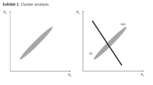
In the first case, if the two variables are very highly correlated, a plot of the two variables would look like Exhibit 1, Panel 1—a tightly grouped set of points that stretch outward from the origin at a 45-degree angle. Of course, if the variables had a very high negative correlation, the same tight grouping would be perpendicular to the original direction. For the sake of this discussion, I will consider only positive correlations, with the understanding that the results will be similar for negative correlations. In Exhibit 1, Panel 1, the tightness of the clustering will depend on the magnitude of the correlation with perfect correlation producing a straight line.

Cluster analysis on two variables is a two-dimensional problem. However, when the two variables are perfectly correlated (to form a straight line when plotted), it becomes a one-dimensional problem. Even when the correlation is not perfect (as in Exhibit 1), it is much closer to a one-dimensional problem than a two-dimensional problem.

If a cluster analysis is conducted on these two variables, the two variables probably will have similar values in each of the clusters. For example, a two-cluster solution can be envisioned by setting a cutting plane at the middle of the data distribution, perpendicular to the long axis (Exhibit 1, Panel 2). This will produce two clusters, one with high values on both variables and the other with low values on both variables.

Similarly in a three-cluster solution, the three clusters will have high values on both variables in one cluster, low values on both variables in the second cluster, and moderate values on both variables in the third cluster. Increasing the number of clusters will keep extending this pattern, producing clusters that aren’t particularly descriptive. If the data are one dimensional, then by definition it should not be possible to get any clusters where the variables have differing values.

Now consider the case where the two variables are uncorrelated as shown in Exhibit 2, Panel 1. The data have a near random pattern because the correlation is very small. If the two variables have zero correlation, the data would have a completely random pattern. The data in Exhibit 2 are without a doubt two-dimensional. If these data are subjected to a cluster analysis, we can easily envision two perpendicular cutting planes dividing the data into four groups with the variable values as high-low, low-high, high-high, and low-low (Exhibit 2, Panel 2). This type of solution would be much more practical than the previous one.

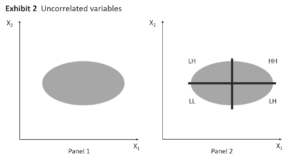
Dimension reduction also implies information reduction. That is, the more variables we have to describe a person, the better our description is. As we strip away each variable, the description of the person becomes less clear. Some types of analysis (e.g., factor analysis) are explicitly used in situations where there are too many variables and dimension reduction is the objective. But this is not the case with segmentation analysis. When some of the variables are highly correlated, they don’t add anything unique to the description of the segments. Hence, collinearity can cause dimension/information reduction and result in segment descriptions that aren’t as rich as they could have been.

Simulation

In order to test if these conclusions are valid, I ran a simulation that used a data set with three normally distributed variables (X1 – X3) and 1,000 observations. The variables were created in such a way that X1 and X2 are highly correlated (.91) and the other two correlations are very low (.08 and .09). All of the variables range from approximately -3 to + 4 in value, with mean values of zero and standard deviations of one.

First, I conducted k-means cluster analysis using SAS with variables X1 and X2. This method was chosen because it is commonly used and well-understood. It uses Euclidean distance measures to calculate the distance between observations in multidimensional space. Depending on the number of clusters requested, a certain number of observations are chosen as cluster “seeds.” Observations closest to a particular seed are grouped together into a cluster. This is followed by an iterative process of calculating the cluster means and (if required) reassigning observations to clusters until a stable solution is reached.

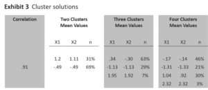
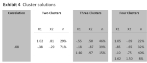
Cluster solutions for two, three, and four clusters were obtained and the results are shown in Exhibit 3. The pattern of means is as expected, given the very high correlation between the variables. That is, both X1 and X2 have high, low, or moderate values within each segment. Next, I conducted the same analysis using X1 and X3, which have a correlation of 0.08. Solutions from two to four clusters are shown in Exhibit 4. The four-cluster solution produces the predicted pattern (high-low, low-low, low-high, and high-high).

In the three-cluster solution, the two largest clusters have substantially different means. The two-cluster solution isn’t much different from the high correlation case, except for a slightly higher difference between the means. This is to be expected because in Exhibit 1, regardless of where the cutting plane is placed, the two variables are going to have about the same mean values on each side of the plane. When the analysis is extended to include five-, six-, and seven-cluster solutions also, the pattern of mean values doesn’t vary much.

Regardless of the number of clusters we choose to look at, the correlation between the two variables results in a predictable pattern of mean cluster values. At very high correlations, mixed value clusters are absent and appear (as very small clusters) only by increasing the number of clusters. At very low correlations, mixed-value clusters dominate in terms of size in solutions with a few clusters, and in terms of number in solutions with more clusters.

The reasoning and simulations used only two variables because of the ease of explanation and graphical representation. But the results can be translated to any number of variables. When variables are highly correlated, it becomes virtually impossible to form clusters where one variable can have a high value and the other can have a low value. It may be possible to do so if a very high number of clusters are derived or if clusters are very small, but practicality would rule out that option. In practice, good segments often are those that have a mixture of high, low, and moderate values on different variables. This makes high correlations problematic.

High Correlation Defined

The simulation looked at extreme values for the correlation coefficients (either lower than 0.10 or higher than 0.90). In practice, what threshold values of correlation coefficients may lead to problems in analysis? One way to test this would be to run simulations such as those described above with varying levels of the correlation coefficients to observe the changes in the types of clusters formed. As before, we need to assume that good segments are those where mean values of variables tend to be different (i.e., high/low, moderate/high, low/moderate as opposed to high/high or low/low). If we can make this assumption, then the simulations may be able to show us the level of correlation below which good segments are likely to occur with increasing frequency.

For this purpose, I created 20 datasets with varying levels of correlation ranging from .95 to .01. K-means cluster analysis was used to provide three- to seven-cluster solutions. Similar patterns arise in all cases. When the correlation between X1 and X2 decreases, mixed-value clusters appear with increasing frequency and size.

The exact results vary somewhat in each solution, but looking at a range of solutions it appears that mixed-value clusters are more likely when correlations are at .50 or lower and are particularly large (or frequent) when correlation values are under .20. Therefore, we could say that, in the context of cluster analysis, high correlation would be above .50 and low correlation would be below .20.

Of course, this demonstration is based on a simulation using just two variables and one clustering method, so the results should be taken as a broad guideline rather than a specific recommendation. The larger lesson here is that higher levels of correlations among variables can cause problems in segmentation analysis and need to be dealt with if the analysis is to proceed smoothly. A more comprehensive analysis is required to fully substantiate the results from this study.

How to Get Past It

Two types of attributes can cause collinearity problems in segmentation that use cluster analysis: irrelevant and redundant attributes. Irrelevant attributes that contribute to collinearity have to be dealt with before starting the analysis. A good understanding of the objectives of the analysis and how the results will be used helps researchers identify the appropriate variables to use in the analysis. Otherwise the tendency is to go on a fishing expedition with all available variables. In such cases, it’s not clear which variables are irrelevant and it’s very difficult to eliminate those variables. Elimination of irrelevant variables is a good reason to start a segmentation analysis with a clearly defined objective. The problem of redundant attributes is exactly the same as multicollinearity in key driver analysis and can be dealt with using the following methods.

Variable elimination: In practical marketing research, quite frequently questions are constructed that tap into very similar attitudes or slightly different aspects of the same construct. Individually, such questions usually don’t provide any additional independent information. The simplest approach for dealing with this situation, if the correlations are very high (e.g., .80 or higher), is to eliminate one of the two variables from the analysis. The variable to be retained in the analysis should be selected based on its practical usefulness or actionability potential.

Factor analysis: Factor analysis can help identify redundancies in the input data set because correlated variables will load highly on the same factor. However, using the factor scores directly as input into a cluster analysis usually isn’t recommended because the nature of the data changes when factor analysis is applied. It’s possible to eliminate some variables that load on the same factor by selecting one or two variables to “represent” that factor. One situation where the use of factor analysis isn’t a problem is when the sample-based segmentation scheme is used for classifying the universe on the basis of variables not used in the analysis.

Variable index: Another method is to form variable indices by combining variables in some form. For example, three highly correlated variables could be averaged to form a composite variable. A more sophisticated method would be to use either exploratory or confirmatory factor analysis to unequally weight the variables and form a composite variable. In this case, essentially, a new construct is being created by explicitly acknowledging its presence in the data in the form of collinearity. While this method eliminates collinearity, the new construct formed must be well understood in order to interpret the results of the segmentation study accurately.

Use a different distance measure. A more complicated approach to the problem is to use Mahalanobis distance measures rather than the traditional Euclidean distances to calculate the closeness of observations in multidimensional space. The Mahalanobis distance is the same as the Euclidean distance when the variables in the data are uncorrelated. When data are correlated, Euclidean distance is affected, but Mahalanobis distance is not. This makes it an attractive candidate for segmentation using collinear variables. However calculation of the Mahalanobis distance measure, especially when there are more than a few variables can be a complicated, time-consuming, iterative procedure.

Use a different method. So far I’ve addressed the problem of collinearity in a Euclidean distance-based method (cluster analysis). But other methods of segmenting data (e.g., latent class segmentation, self-organizing maps (SOM), and tree-based methods, such as CHAID) may not be susceptible to this problem.

Latent class segmentation is a model-based method that uses maximum likelihood estimation to simultaneously segment the data as well as run regression models for each segment.

Collinearity could be a problem in the regression models, but it’s not clear how much of a problem it would be in the formation of the segments. SOM is a neural network that makes virtually no assumptions about the data. While its reliance on Euclidean distances for creating a topological map could make it vulnerable to collinearity problems, other available distance measures may alleviate the problem. Methods such as CHAID rely on splitting variables one at a time and hence may not be susceptible to collinearity problems. However, without a thorough investigation, it’s impossible to say all these methods are free of collinearity problems, even though it does appear that, in theory, the problem should be less severe than in cluster analysis. Segmentation by itself is a long and arduous process requiring choices to be made based on study objectives, type of data, analytical method, and guidelines for decision criteria. It doesn’t need to be further complicated by the presence of collinearity in the data when cluster analysis is used to create the segments. While it is true that practical segmentation studies almost always use more than two variables, I hope the information from this study will lead to a better understanding of the problems caused by collinearity and possible solutions. Of course, this preliminary effort needs to be expanded in scope to properly understand the role of collinearity in segmentation problems